
Testing Part 5: Exposure Features
by Kevin Garwood
| Testing Overview | Previous | Next |
Background
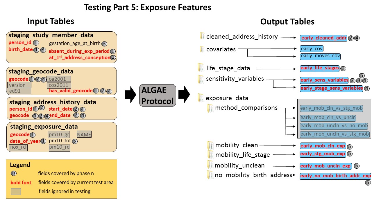
These features are used to assess exposures in one of four ways. In the cleaned mobility assessment , aggregated life stage exposures are calculated based on contributions of all address periods that fall within the study member's exposure time frame. The uncleaned mobility assessment considers the contributions of all relevant address periods, but ignores exposures from days that have been involved in a gap or an overlap between successive address periods. In the life stage mobility assessment, the location study members occupied on the first day of each life stage is used to represent the location for the entire stage. The early life analysis has one more assessment approach than the later life analysis. The birth address assessment uses the address at birth to represent for the entirety of the study member's exposure time frame.
Initially, early life analyses used daily exposure records while later life analysis used weighted annual exposure values. The differences in exposure inputs warranted having test suites designed to test the protocol in early and later life analyses. However, later on the protocol code was changed so that both analyses would aggregate daily exposure records. In the case of the later life analysis, weighted annual values were used to generate exposure values for every day of every year that was covered in the analysis. Once daily exposure values have been generated, the early and later life analyses used identical code to process exposures.
Although the two analyses use almost exactly the same code to assess exposures, test suites for early and later life analyses will be retained. Although sharing the exposure assessment code between the two analyses simplified testing, the effect of using daily exposure values for the later life analysis has greatly increased the amount of time needed to run the protocol. In future, the code used to assess later life exposures may once again be changed to improve performance. Therefore, we are preserving early and later life test suites just in case the code for supporting early and later life analyses diverges again.
This is the most complex and labour intensive area of testing for the whole project. Fake exposure data had to be generated in a way that made it amenable to manual calculations for each of the exposure assessments. In an effort to minimise testing efforts, we elected not to develop automated test cases for features that compare corresponding results in results that are generated by different pairs of assessment.
Coverage
Input Fields Covered by Test Cases
| Table | Field |
|---|---|
| staging_exp_data | geocode |
| staging_exp_data | date_of_year |
| staging_exp_data | pm10_tot |
Output Fields Covered by Test Cases
| Table | Field |
| early_mob_cln_exp | ith_life_stage |
| early_mob_cln_exp | life_stage |
| early_mob_cln_exp | pm10_tot_sum |
| early_mob_cln_exp | pm10_tot_avg |
| early_mob_cln_exp | pm10_tot_med |
| early_mob_cln_exp | pm10_tot_err_sum |
| early_mob_cln_exp | pm10_tot_err_med |
| early_mob_cln_exp | pm10_tot_err_avg |
| early_mob_uncln_exp | ith_life_stage |
| early_mob_uncln_exp | life_stage |
| early_mob_uncln_exp | pm10_tot_sum |
| early_mob_uncln_exp | pm10_tot_avg |
| early_mob_uncln_exp | pm10_tot_med |
| early_stg_mob_exp | ith_life_stage |
| early_stg_mob_exp | life_stage |
| early_stg_mob_exp | pm10_tot_sum |
| early_stg_mob_exp | pm10_tot_med |
| early_stg_mob_exp | pm10_tot_avg |
| early_no_mob_birth_addr_exp | ith_life_stage |
| early_no_mob_birth_addr_exp | life_stage |
| early_no_mob_birth_addr_exp | pm10_tot_sum |
| early_no_mob_birth_addr_exp | pm10_tot_med |
| early_no_mob_birth_addr_exp | pm10_tot_avg |
Test Case Design
Ignore features that compare results from different pairs of assessment methods
ALGAE automatically compares results between various pairs of exposure assessment methods. These appear in themethod_comparisons directory of the results file folder.
Because of limited resources, these have not been tested.
All calculations for percent error are done by the function:
calc_percent_error(exact_value, approximate_value);, which was tested with
ad hoc values.
Use only one pollutant for testing
ALGAE treats all pollutant values exactly the same. Therefore, for the purposes of testing, only one pollutant needs to be used to check that exposure calculations are working correctly.Engineer exposure data so they are easy to calculate
In real-world scenarios, the concentration of a pollutant will rise and fall in response to various complex factors. In the test data, the concentration of each pollutant remains permanently fixed at each geocode. The constant value of a pollutant from day to day at a given location makes exposure assessments easier to calculate by hand.Engineer the daily exposure data so that each pollutant type produces very different results
Although onlypm10_tot is used in exposure test cases, fake data values for
the other pollutants have been designed to guarantee that results will significantly vary
between one pollutant type and another. The design of the other pollutant values is meant to
make it easy to identify errors where the code is using the wrong pollution type for a
calculation (eg: it's using the same field for nox_rd and pm10_tot.
Engineer daily exposure data to make it easier to see mistakes in exposure error assessment
In ALGAE, exposure error is assessed as the difference between the pollution between the location assigned by data cleaning and the opportunity location that may have otherwise been used for assessment. In order to make it easy to know that that the correct assigned and opportunity geocodes are being used, the pollutant values are stepped at each location for each day. The data table below shows how pollution values are stepped between locations and between pollutants.Geocode PM10_rd nox_rd pm10_gr name pm10_tot a1 1.0 2.0 3.0 4.0 5.0 a2 3.0 4.0 5.0 6.0 7.0 a3 6.0 7.0 8.0 9.0 10.0 a4 10.0 11.0 12.0 13.0 14.0 a5 15.0 16.0 17.0 18.0 19.0 a6 21.0 22.0 23.0 24.0 25.0
Values vary across pollutants to produce obviously different exposure results,
but only pm10_tot is used in test cases. For pm10_tot,
the concentrations vary in a sequence of +2.0, +3.0, +4.0, +5.0, +6.0... in
order to ensure that the difference between any two successive locations will
be different. For example, if the study member moves from a3 to
a4, the exposure error measured between these locations will be
different than if the a3 was used with any other location.